Graph Convolutional Networks

Graph Convolutional Networks (GCN)

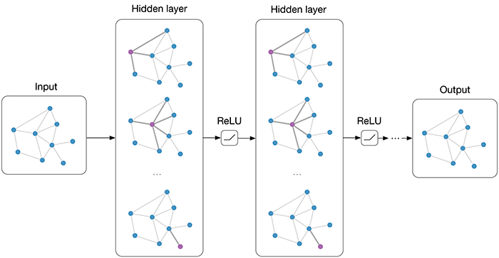
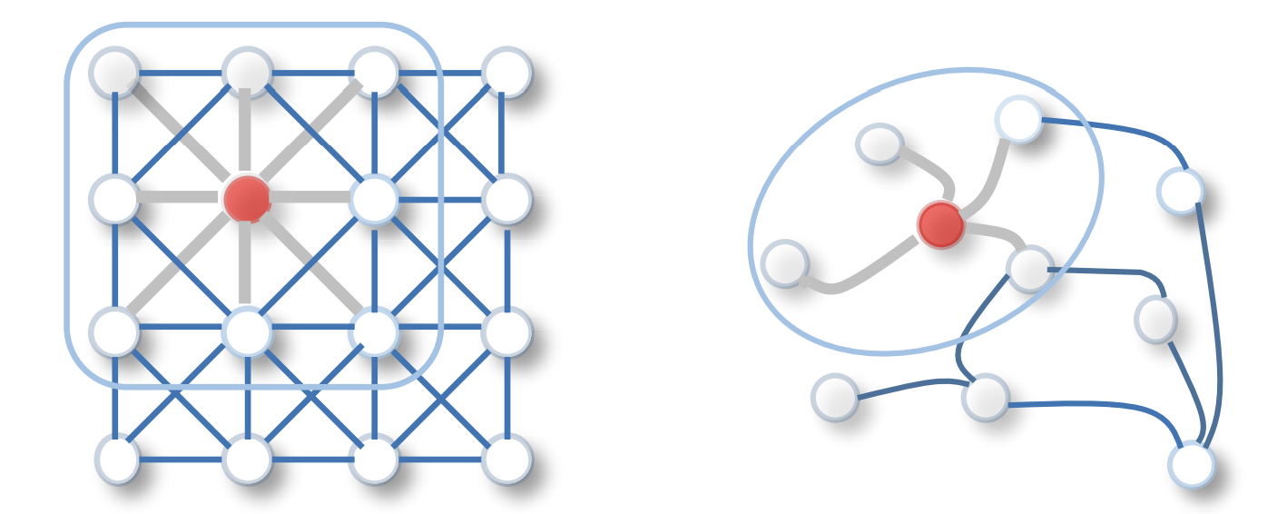
The general idea of GCN is to apply convolution over a graph. Instead of having a 2-D array as input, GCN takes a graph as an input.

Many problems are graphs in true nature. In our world, we see many data are graphs, such as molecules, social networks, and paper citations networks.

A graph (directed or undirected) consists of a set of nodes and a set of edges E.
Nodes are represented by attribute values (can be scalar or vector) (the data of nodes)
Edges can be weighted (weights can be scalar or vector) or binary (structure of the graph).

GCNs can be categorized into 2 major algorithms, Spatial Graph Convolutional Networks and Spectral Graph Convolutional Networks.
we will focus on Fast Spectral Graph Convolutional Networks.

The original idea behind Spectral GCN was inspired by signal/wave propagation.
We can think of information propagation in Spectral GCN as signal propagation along the nodes.
Spectral GCNs make use of the Eigen-decomposition of graph Laplacian matrix to implement this method of information propagation.
To put it simply, the Eigen-decomposition helps us understand the graph structure, hence, classifying the nodes of the graphs.
This is somewhat similar to the basic concept of Principal Component Analysis (PCA) and Linear Discriminant Analysis (LDA) where we use Eigen-decomposition to reduce dimensionality and perform clustering.
In this approach, we will take into account the Adjacency Matrix (A) in the forward propagation equation in addition to the node features (or so-called input features).
A is a matrix that represents the edges or connection between the nodes in the forward propagation equation.
The insertion of A in the forward pass equation enables the model to learn the feature representations based on nodes connectivity.

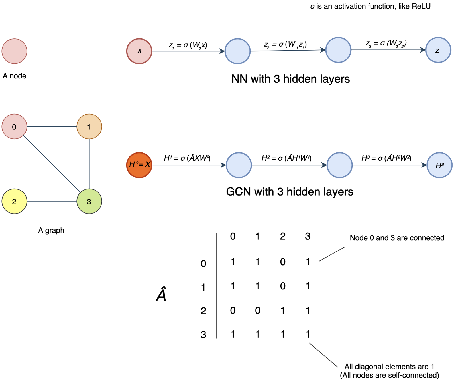
The first diagram (the first row) below is the NN as we know and the second diagram is the GCN with a graph containing four nodes as the input.

In the first NN, it contains multiple dense layers (fully connected layers).
x is the input for the first layer and zᵢ is the output of layer i.
For each layer, we multiple z (or x for the first layer) with the weight matrix W and pass the output to an activation function σ, say ReLU.

GCN is very similar, but the input to σ is ÂHⁱWⁱ instead of Wᵢzᵢ.
i.e. σ(Wᵢzᵢ) v.s. σ(ÂHⁱWⁱ) where zᵢ and Hⁱ are the output vectors from the last hidden layer for NN and GCN respectively.
But please note that Wⁱ and Wᵢ are different and have different dimensions. And for the first layer in GCN, X contains an array of nodes instead of a single node x. X will be encoded as a matrix with each row contains the features of a node.

So what is Â? GCN introduces an adjacency matrix A as shown before.
The element Aᵢⱼ in A equals 1 if node i and j are connected. Otherwise, it will be zero. So Â indicates the neighbors of a node.
But we will make one more adjustment to indicate all nodes are self-connected.
This indicates the output of a node in a hidden layer depends on itself and its neighbors.
So, we convert all diagonal elements of A to 1 to form Â. Mathematically, Â equals A + I.

That comes to the output of the hidden layer to be σ(ÂHⁱWⁱ).
If we ignore W for a second, for each node in a hidden layer, ÂHⁱ sums up features on each node with its neighbors.

However, we may face the vanishing or exploding problem in a NN if we don’t have certain control over the range of the hidden layer output.
In specific, GCN wants Â to be normalized to maintain the scale of the output feature vectors.
One possibility is to multiple Â with D̂⁻¹ where D̂ is the diagonal node degree matrix of Â in measuring the degree of each node.
At a high level, instead of summing up itself with its neighbor, multiplying the sum with the inverse D̂⁻¹ sort of averages them.
Specifically, D̂ is a diagonal matrix with each diagonal element D̂ᵢᵢ counts the number of edges for the corresponding node i. And the output for each hidden layer becomes σ(D̂⁻¹ÂHⁱWⁱ), instead of σ(ÂHⁱWⁱ).

Let’s calculate D̂ in our example. For an undirected graph, the degree of a node is counted as the number of times an edge terminates at that node. So a self-loop will count twice.
In our example, node 0 has 2 edges connecting to its neighbors plus a self-loop. Its degree equals 4 (i.e. 2 + 2). For node 3, its degree equals 5 (3 + 2).

And D̂⁻¹ equals

The diagram below summarizes the model discussed so far. In this example, it has 3 hidden layers and for each hidden layer, it computes its output as σ(D̂⁻¹ÂHⁱWⁱ).

In the main paper, Kipf and Welling states that doing symmetric normalization will make dynamics more interesting, hence, the normalization equation is modified from:

https://towardsdatascience.com/understanding-graph-convolutional-networks-for-node-classification-a2bfdb7aba7b (awesome for implemntaion details)
https://towardsdatascience.com/graph-convolutional-networks-on-node-classification-2b6bbec1d042 (awesome for implemntaion details)
https://jonathan-hui.medium.com/graph-convolutional-networks-gcn-pooling-839184205692 (show more details for spatial and spectral GCN and different stuff).

Written on August 14th, 2021 by Islam Mohamed

Feel free to share!